Optimization & Simulation of Power System Expansion Plans
Overview
Program CAPRICORN has been developed by Power & Water Systems Consultants. (PWSC) to optimise and simulate the expansion of large scale power supply systems.
Development was prompted by the limitations of existing and widely used generation system expansion planning software such as WASP and AS-PLAN, including their inability to:
model transmission systems and hence multiple demand areas;
mathematically guarantee the optimum selection and introduction of hydroelectric plants;
cater for project interdependencies.
CAPRICORN consists of an Optimisation Module and a Simulation Module, which share a common set of data input files.
The Optimisation Module employs Mixed Integer Linear Programming (MILP) to simultaneously optimise the scheduling of generation plant, transmission lines, and import and export quantities, while taking account of project interdependencies, demand management and budgetary constraints.
The Simulation Module uses Linear Programming (LP) to determine the least cost load dispatch in each month of a simulated expansion plan, taking account of constraints on generating plant outputs, transmission load flows, transmission losses, and demand dependent supply benefits and deficit penalties. Deterministic or probabilistic simulations can be performed, and operating cost estimates provided for renewable energy plant outputs associated with up to 5 Hydrological Conditions. Investment and operating costs are accounted on a monthly basis.
CAPRICORN's Graphical User Interface provides facilities for the:
editing of data input files;
interactive definition of alternative expansion plans;
display of detailed and consolidated results in graphical and tabular form, and their export in CSV format output files;
Input operating and investment cost data used by CAPRICORN to optimise and simulate the performance of an expansion plan are input via the Catalogue Data (*.CAT) file and include:
for hydroelectric plants - fixed operation and maintenance (O & M) costs ($/month), variable operating costs ($/MWh and $/MW), economic lifetime (months), and monthly investment costs split into local, foreign and labour components (million$);
for thermal plants - fixed O & M costs ($/month), variable operating costs at and above Minimum Stable Load ($/MWh), capacity costs ($/MW), economic lifetime (months), and monthly investment costs split into local, foreign and labour components (million$);
for transmission lines - fixed O & M costs ($/month), variable operating costs ($/MWh and $/MW), economic lifetime (months), and monthly investment costs split into local, foreign and labour components (million$).
Technical data considered during the load dispatch optimisations include:
for hydroelectric and wind plants - installed (maximum) capacity (MW), 'firm' and average annual energy production (GWh) or calendar monthly plant availabilities in terms of MW and GWh (by hydrological condition), forced outage rate (%);
for thermal plants - installed (maximum) capacity (MW), Minimum Stable Load (MW), maximum and minimum annual energy production (GWh) or calendar monthly availabilities in terms of MW and GWh, forced outage rate (%);
for transmission lines - maximum carrying capacity (MW), forced outage rate (%), and loss factor (%).
For hydro plants, up to five 'hydrological conditions' can be considered, with different calendar monthly power and energy availabilities being assigned to each condition. Their 'probabilities of occurrence' may, for example, be associated with 'very dry', 'dry', 'average', 'wet' and 'very wet' conditions, thereby providing consistency with data inputs to the WASP and A/SPLAN programs.
If only annual values for 'firm' and average energies are input, these are automatically pro-rated within CAPRICORN to give the requisite monthly values for the 'very dry' ('firm') and 'average' hydrological conditions. Monthly non-hydro plant availabilities can be used to take account of planned maintenance schedules.
The optimal role of individual hydro plants will often vary with the development of an integrated electricity supply system and CAPRICORN simulation module allows monthly hydro plant capabilities to be varied as a function of the expansion plan year.
This facility can be particularly pertinent when optimising the development of systems which include non-hydro forms of generation, such as wind and solar, which have significant seasonal availability constraints. Such data can be provided directly by PWSC's AQUARIUS program.
The demands associated with each demand centre in the system are given in terms of the load in MW for each of up 8 blocks, and the duration of each block given in hours. These loads can be varied as a function of hydrological probability, thus enabling the modelling of preventive rationing or demand management. For example, the demands to be met can be reduced by a specified amount in the event of 'very dry' hydrological conditions being experienced.
Differential unit prices for supplied energy and costs of unserved energy can be associated with each individual electricity demand centre modelled.
The Expansion Plan Optimization module employs a Mixed Integer Linear Programming (MILP) algorithm to optimize the commissioning dates of all candidate generation plants, transmission lines, as well as import and export quantities, consistent with meeting forecast electricity demands at least net cost over a given planning period.
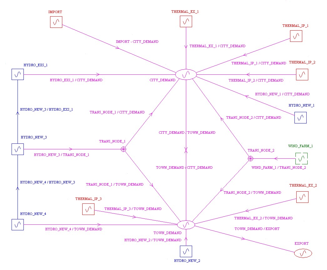
Figure 1 : Demonstration System used to Develop the CAPRICORN Optimization Module
The theoretical system used in developing the Optimisation Module shown as Figure 1 features a variety of options for expanding the system that initially consists of hydro plant HYDRO_EXS_1 and thermal plant THERMAL_EX_1 supplying CITY_DEMAND, and thermal plant THERMAL_EX_2 supplying TOWN_DEMAND via existing transmission lines.
In this example, development options include:
interconnecting CITY_DEMAND and TOWN_DEMAND;
importing electricity via a connection to CITY_DEMAND;
exporting electricity via a connection from TOWN_DEMAND;
alternative transmission routes (e.g. connecting WIND_FARM_1 to CITY_DEMAND via transmission line TRANS_NODE_2 / CITY_DEMAND or to TOWN_DEMAND via transmission line TRANS_NODE_2 / TOWN_DEMAND).
The optimization procedure takes account of:
the technical and economic characteristics of all existing and potential generation plant and transmission lines, including their investment and operating costs, construction periods, maximum and minimum power and energy outputs, etc.;
up to 5 Hydrological Conditions associated with different hydro plant energy availabilities and their associated weighting factors for estimating operating costs, supply benefits and shortage penalties;
differential supply benefits and deficit costs associated with individual electricity demands, including exports;
mutual exclusivities e.g. generation plants THERMAL_IP_1 or THERMAL_IP_2 can be commissioned, but not both;
mutual dependencies e.g. transmission line TRANS_NODE_3 / CITY DEMAND cannot be commissioned before transmission line HYDRO_NEW_3 / TRANS_NODE_3;
project interdependencies e.g. as a result of improved flow regulation, commissioning of hydro plants HYDRO_NEW_3 or HYDRO_NEW_4 will improves the energy capabilities of the existing hydro plant HYDRO_EXS_1;
annual cost (budget) constraints associated with combinations of investment costs, operating costs, deficit penalty costs, and supply benefits; specified economic parameters including discount rates and variable operating (fuel) cost inflation rates.
Within the Linear Programming formulation Commissioning Variables (CV's) are used to determine, for each step of the expansion planning period, the optimal fraction of the available maximum capacity of a candidate generation plant or transmission line to be introduced into the system or the demand to be supplied. As is normal, the linear programming optimization algorithm first establishes a 'continuous' solution in which the CV's can take any value between 0 and 1, while the sum of the CV's associated with each component must be <= 1. If specified, the solution algorithm then imposes constraints that the CV's can only take binary values i.e. 0 or 1, so that components can be commissioned in their entirety (maximum capacity) or not at all.
For any run, the user can stipulate individually whether hydro plant, thermal plant, transmission line or demand areas CV's are to be restricted to binary values.
It can be noted that the continuous LP solution can often provide valuable information regarding the optimal dimensioning and phased introduction of individual components. For thermal plant installations, the facility is available to limit the maximum capacity increment, in MW, that may be commissioned in consecutive time steps.
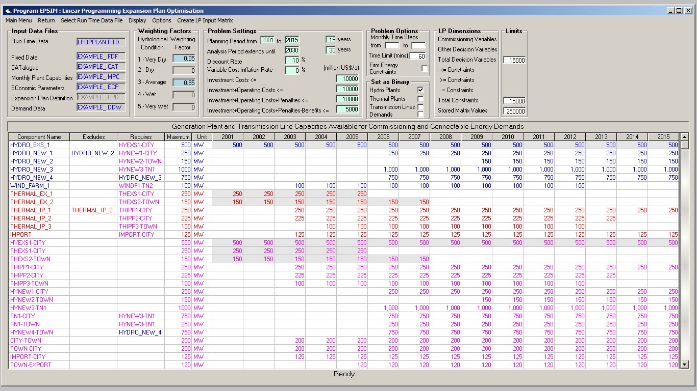
Following reading of the CAPRICORN input files, the optimisation problem is presented in the form shown in Figure 2 below.
Figure 2: Demonstration Problem Representation
The screen shows the names of the selected input files, the Hydrological Conditions to be considered and their associated operating cost weighting factors, the planning period (in this case from 2001 to 2015), the period of analysis (in this case an additional 15 years), the discount and annual operating cost inflation rates to be applied, and the annual limits on investment, investment + operating costs, investment + operating costs + deficit penalties and investment + operating costs + deficit penalties - supply benefits (net costs).
The screen allows the user to set a maximum time limit for the LP solver to find the optimal solution and individually force the Commissioning Variables for hydro plants, thermal plants, transmission lines and demands to be binary i.e. 0 or 1.
The names of the existing and candidate hydro plants (blue), thermal plants (red), transmission lines (magenta) and electricity demand centres (green) are listed in Column 1 of the table, which also shows any associated mutual exclusivities (Column 2), dependencies (Column 3) and maximum capacities in MW or energy demands in GWh.
For each time step of the planning period, and each generation plant and transmission line, the table indicates the capacity available for commissioning, taking account of specified construction times. A grey background is used to indicate that a component is already present or that its commissioning date is fixed.
For each electricity demand area and each planning step, the table shows the forecast energy demand in GWh and a grey background shows that a demand area is already in the system. Finally, the least two rows of the table indicate the total potential energy demands and energy generation in each time step.
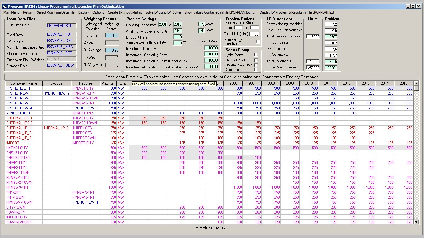
The linear programming input matrix is generated when the 'Create LP Input Matrix' option is pressed on the Top Menu of the screen and, as shown below, the resulting dimension are shown in terms of the number of Commissioning Variables, the number of other decision variables, the total number of decision variable, the number of <=, <=, and = constraints, and the total number of constraints.
Figure 3: Demonstration Problem Linear Programming Input Matrix Dimensions
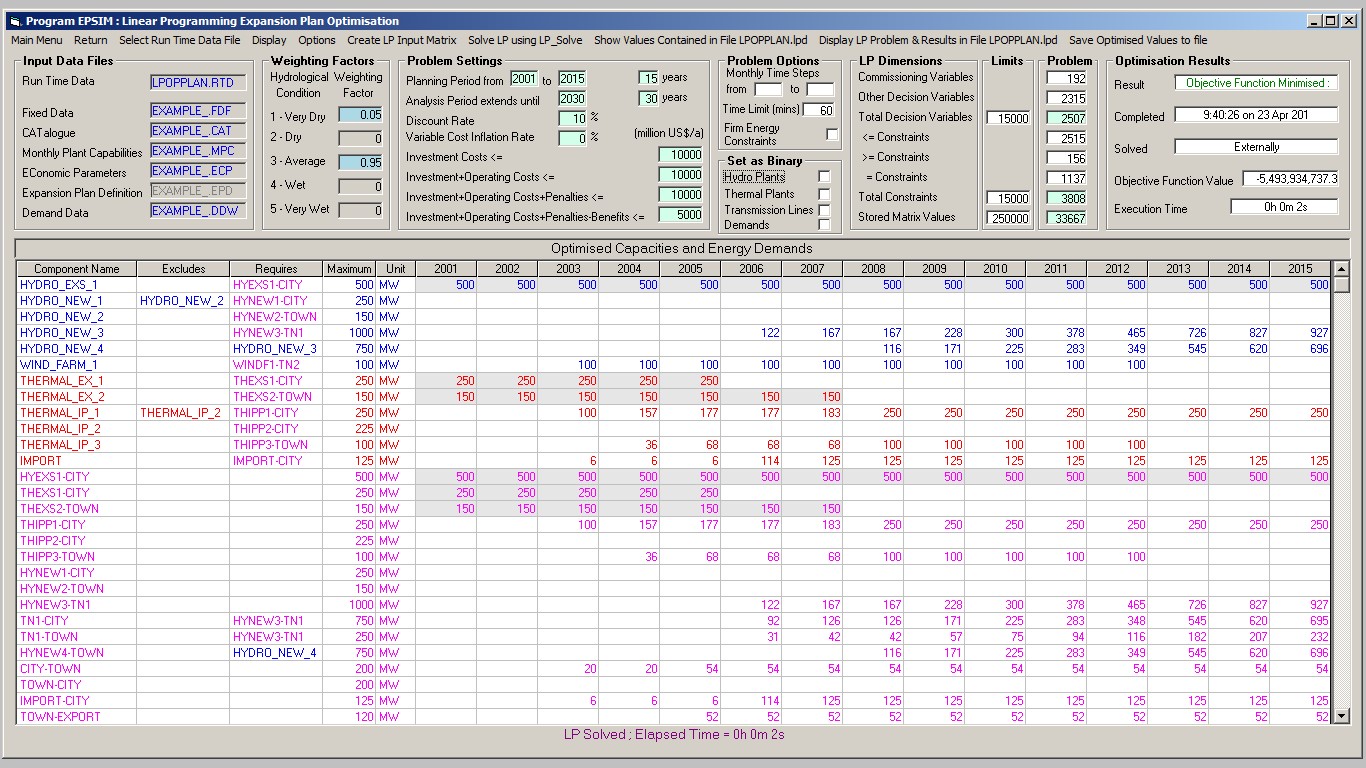
Figure 4 below shows the optimum expansion plan obtained by solving the demonstration problem without imposing binary conditions on any Commissioning Variables.
Figure 4: Continuous Linear Programming Solution of Demonstration Problem
The optimised value of the objective function is shown to be -5,493,934,737.3 with a solution time of just 2 seconds. It can be noted that the objective function value is negative since, as shown, in most years of the planning period the electricity supply benefits exceed the total investment, operating and deficit penalty costs.
The table shows that, as can be expected, several system components would ideally be commissioned in stages, although there are a number of exceptions including, for example, WIND_FARM_1 and exports at the maximum of 438 GWh per year.
The table also shows that the optimal solution has no associated deficit penalties.
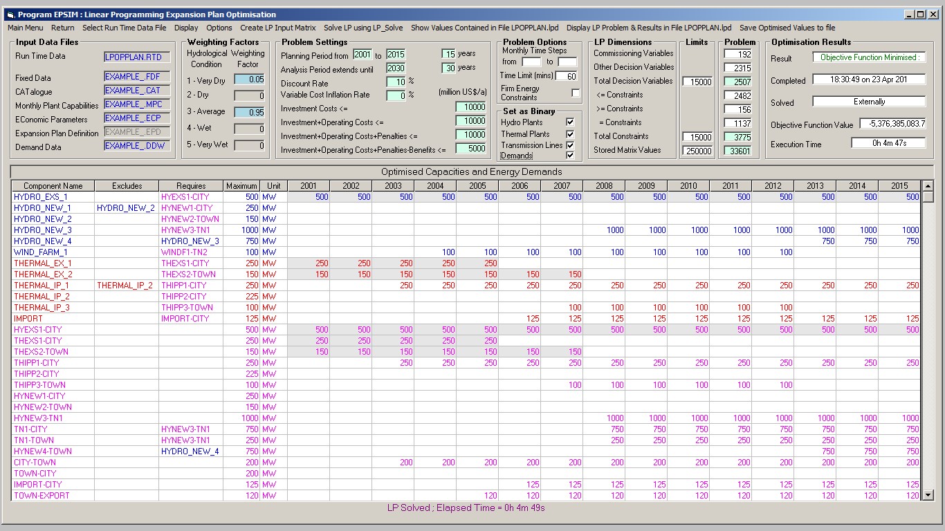
Figure 5 : Mixed Integer Linear Programming Solution of Demonstration Problem
Figure 5 shows the optimal solution obtained if all hydro plants, thermal plants, transmission lines and connectable demand areas CV's are constrained to take binary values.
As is to be expected, imposition of these constraints results in an increase in the optimised value of the objective function to -5,376,385,083.7, compared with -5,493,934,737.3 for the continuous solution. It can also be noted that the solution time is considerable longer at 4 minutes and 49 seconds.
The table shows that, as specified, all system components are commissioned in their entirety i.e. with their maximum installed capacities, or not at all.
The total installed firm energy is less than the demand in the years 2010, 2011 and 2012, and that as a result deficit penalties are incurred in years 2009 to 2012.
It can also be observed that although the installed 'firm' (Hydrological Condition 1) energy significantly exceeds the total demand in 2009, a small deficit is shown as a result of transmission losses and load flow constraints.
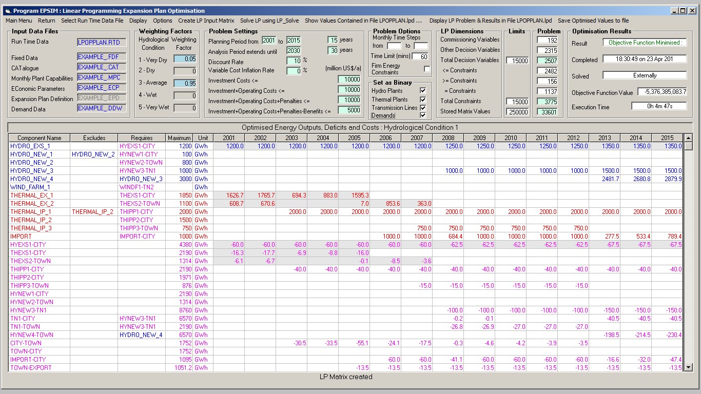
Figure 6 : Mixed Integer Linear Programming Solution Energy Outputs and Losses Hydrological Condition 1
Figure 6 shows the energy produced by each generation plant and the transmission line losses associated with Hydrological Condition 1 i.e. with available hydro plant energies under 'very dry' conditions.
It can be seen that the total energy supplied is less than the demand in years 2009 to 2012 and that on account of the penalties incurred, the net cost in year 2011 and 2012 is positive i.e. the total investment and operating costs are greater than the supply benefits.
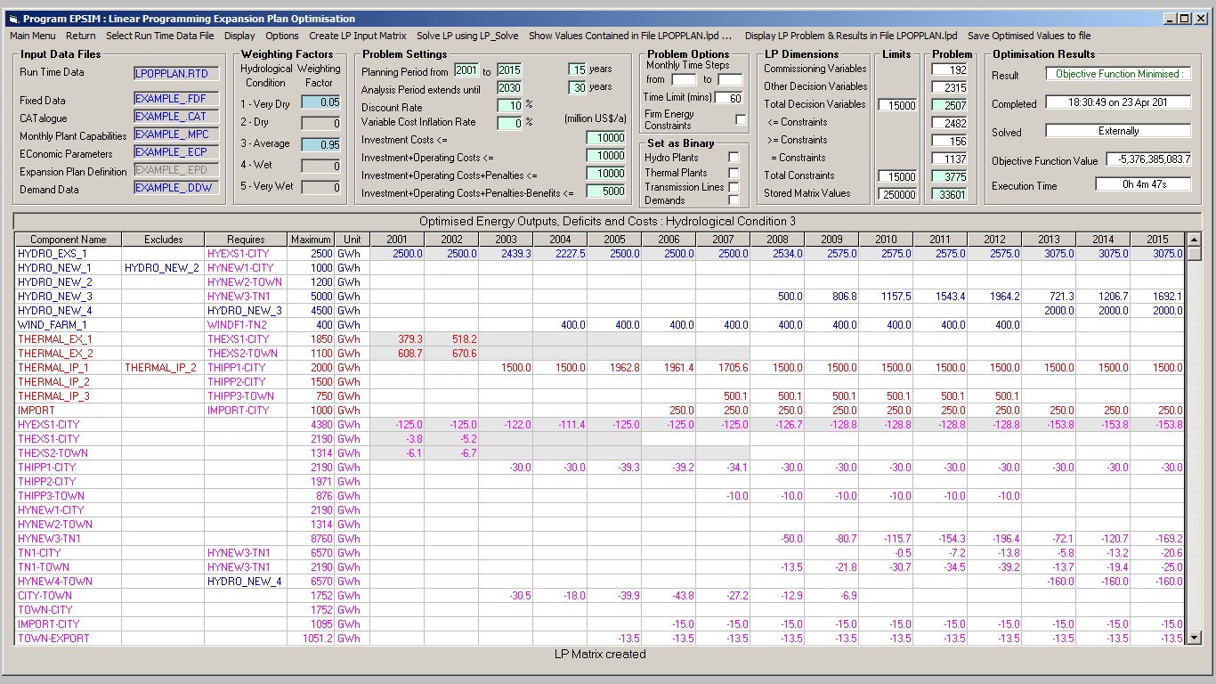
Figure 7 : Mixed Integer Linear Programming Solution Energy Outputs and Losses Hydrological Condition 3
Figure 6 shows the energy produced by each generation plant and the transmission line losses associated with Hydrological Condition 3 i.e. with available hydro plant energies under 'average' conditions.
It can be seen that the total energy supplied is equal to the demand in all years 2009 to 2012 and that the net costs are negative i.e. the total investment and operating costs are less than the supply benefits.
The CAPRICORN Simulation Module simulates the performance of electricity system expansion plans defined by the commissioning and retirement dates (year and month) of system elements, namely hydroelectric plants, non-hydro (thermal, solar and wind power) generation plants, transmission lines and electricity demand areas. Such plans can be manually defined (by editing the appropriate CAPRICORN input file), constructed interactively by selecting from candidate system elements, or generated by an optimisation facility.
With the interactive construction facility the user is provided with guidance regarding the ranking of candidate plants, in terms of $/MW installed, $/GWh (firm), $/GWh (average) etc., the monthly peak load (MW) and energy (GWh) demands to be met, and construction time constraints. Compliance with data specified earliest and latest commissioning dates and economic lifetimes, and mutual exclusivities, are also checked.
Plans can be generated automatically on the basis of $/MW installed, $/GWh (firm), $/GWh (average) and other heuristic ranking indices. On completion, the corresponding commissioning and retirement dates are automatically written to the Expansion Plan Definition (*.EPD) input file.
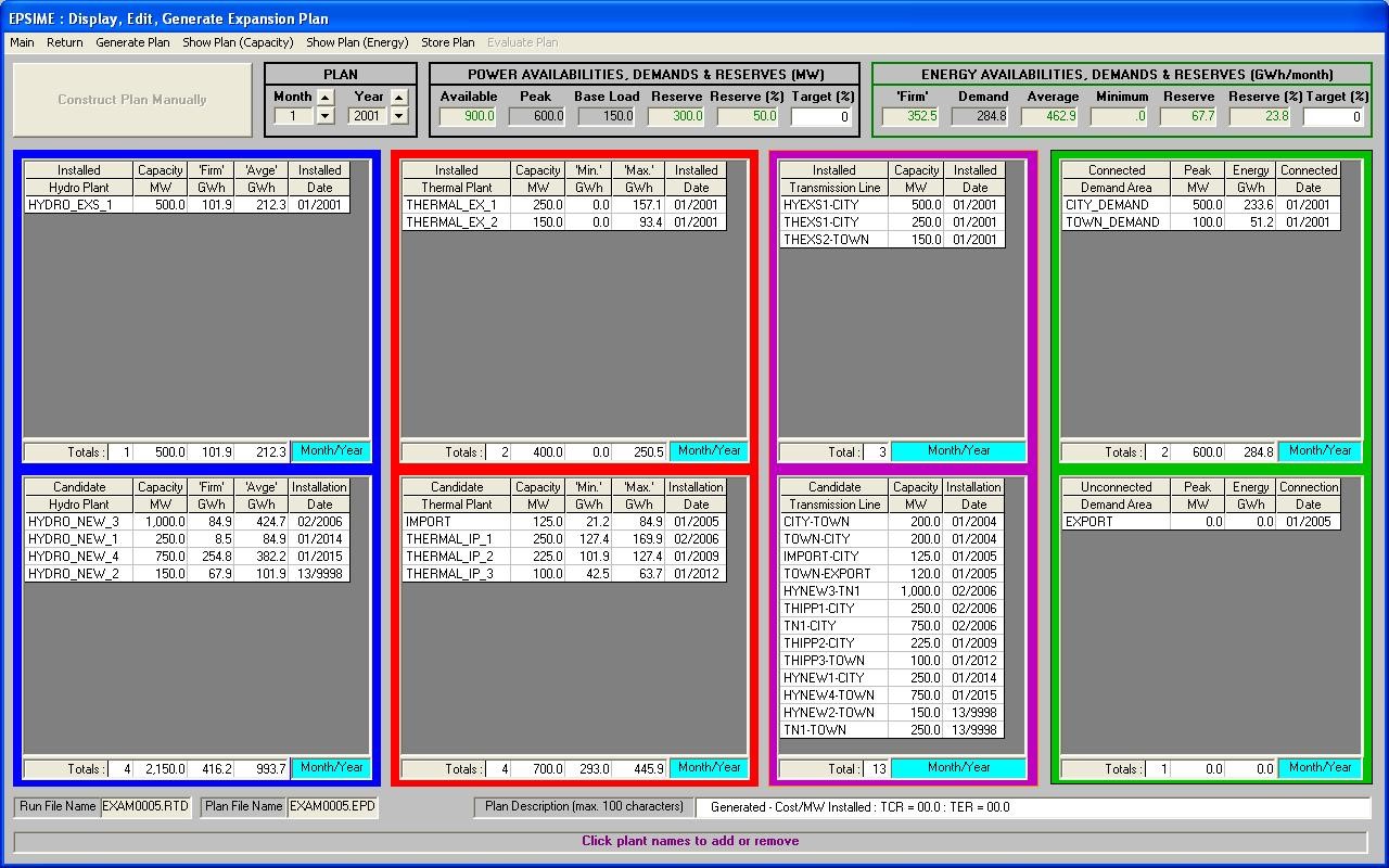
An example of the CAPRICORN screen provided for the display, construction and automatic generation of system expansion plans is shown as Figure 8.
Figure 8 : View, Construct and Generate System Expansion Plan
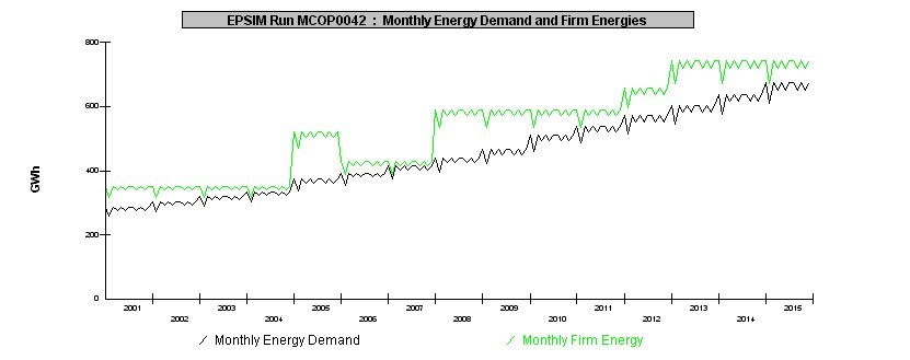
The installed capacity or energy availability associated with a given expansion plan, together with the annual additions and subtractions can be displayed graphically, as shown in Figure 9.
Figure 9 : Monthly Energy Demands, Availability and Annual Totals
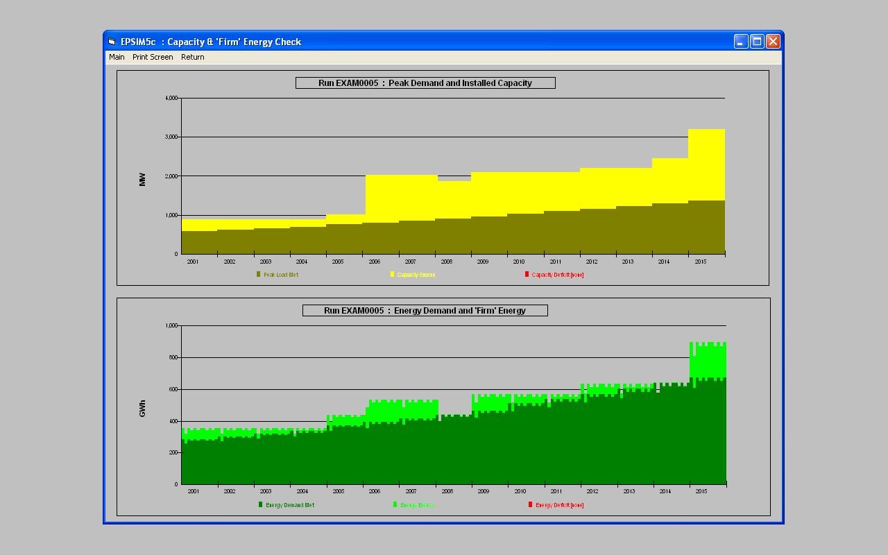
The coverage of forecast peak load and energy demands can be plotted in the form shown in Figure 10 below.
Load dispatch simulations are performed for each month of the specified expansion planning period, taking into account the system composition defined in the *.EPD file. These simulations are used to establish the ability of the defined system configuration to meet the forecast demands for electricity and to estimate the operating costs, including those relating to any unserved energy.
A Linear Programming (LP) formulation is used with the demand specified in blocks representing either the chronological load or the load duration curve and can optionally consider multiple demand areas and transmission constraints/losses, and hence explicitly imports and exports, as well as minimum and maximum monthly power and energy plant outputs. The position of each generating plant in each load block can be identified and optional constraints can be imposed so that the output from each plant must be at least that dispatched in a lower load block.
The load dispatch simulations can be performed in either deterministic or probabilistic mode. In deterministic mode the forced outage rate associated with all system components is assumed to be zero. In probabilistic mode multiple load dispatch simulations are performed, with the capacities of individual and combinations of system components being systematically set to zero. A loss of load probability limit can be set and computed as the product of the individual component forced outage rates, below which the associated load dispatch simulations are suppressed. For each simulation the loss of load (MW) and the corresponding probability are recorded, and any combination of hydro plant, thermal plant and transmission line outages can be specified.
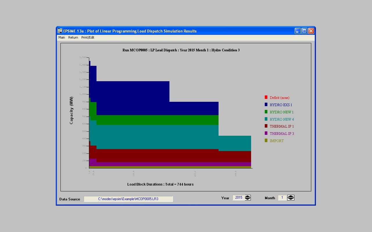
The results of all load dispatch simulations performed are stored in fully annotated output files, one for each hydrological condition specified. The output of each generation plant and associated operating costs in each load dispatch block are given and, if modelling of transmission lines is specified, the tables also indicate for each block the load flow through each line (MW), the energy carried (GWh), losses incurred and the associated transfer costs (if any). The contents of these output files can be displayed in tabular and graphic form to show the production of each plant in each month and load dispatch block. An example of the graphic form is shown in Figure 11 below.
Figure 11 : Monthly Load Dispatch Plot
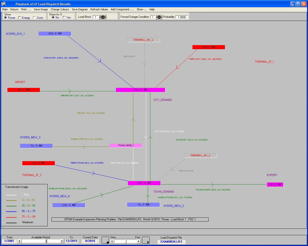
An example of a 'mimic' diagram representation, which can be used to show the status and outputs of system components in any month and load block of the expansion planning period, is given in Figure 12.
Figure 12 : Mimic Diagram Representation of Load Dispatch Results
Graphs can also be produced which show the loss of load probability and either the loss of load (MW) or the loss of energy (GWh) in each month of the planning period. In both cases the facility is provided to 'page through' the planning period month by month. For each alternative expansion plan and hydrological condition, graphical screen and printer outputs can be produced showing:
the monthly peak load and capacity coverage, split between hydro and thermal plants, and with any deficits highlighted;
the monthly energy demand and energy availability, split between hydro and thermal plants, and with any deficits highlighted;
the monthly peak load and dispatched capacity, split between hydro and thermal plants, and with any deficits highlighted;
the monthly energy demand and dispatched energy, split between hydro and thermal plants, and with any deficits highlighted.
Calculation of Present Worth Costs and Sensitivity Analysis
The Present Worth Cost associated with a given expansion plan is computed as the total discounted value of all investment and operating costs, including the cost of supply deficits ($/MWh) and any 'salvage' credits associated with components with an economic lifetime extending beyond the planning period.
The user may also specify an 'evaluation' period longer than the planning period, during which the demand to be met and operating costs are assumed to be the same as for the last year of the planning period.
All expenditures and benefits are accounted for on a monthly basis. In the event of more than one ('average') hydrological condition is analysed, the monthly operating and unserved energy costs are taken to be those associated with each load dispatch simulation weighted by the assigned hydrological probability.
The Present Worth Costs for each expansion plan are calculated for each combination of input ranges of economic parameters, namely:
shadow prices on local, foreign and labour investment costs, and on local and foreign operating costs.
The 'base case' present worth cost associated with each alternative expansion plan is automatically stored within an integrated data base, together with the names of the input data and output files used and supply reliability indicators i.e. the number of months when demand could not be met and, if probabilistic load dispatch is employed, the maximum Loss of Load Probability in any month.
Graphical screen and hard copy outputs can be produced showing the monthly cash flow of investment, operating costs and, optionally, revenues and deficit costs. Total investment costs can be shown or disaggregated into local, foreign and labour components.
The required (constant) price of generated electricity necessary to meet total expenditures over the planning period is also calculated, and the associated net cash flow can be plotted.
The Internal Rates of Return of each generation plant included in a given expansion plan are computed and output to the Expansion Plan Results (*.EOR) file.
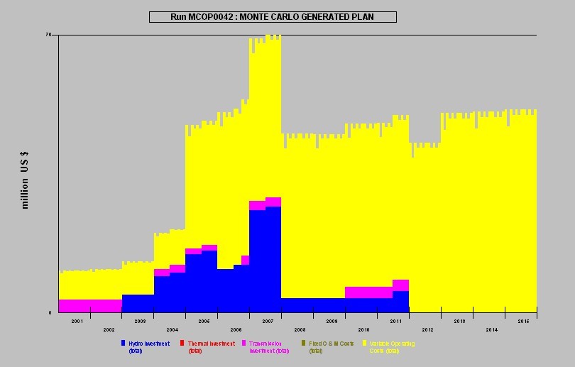
An example plot of total investment and operating costs is shown as Figure 13.
Figure 13 : Plot of Investment and Operating Cost Streams
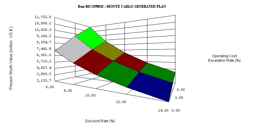
Graphs showing the sensitivity of the PWC to the input ranges of the economic parameters can be displayed and printed, as illustrated in Figure 14 below.
CAPRICORN has been designed to be used either as a 'stand alone' expansion planning tool, or to refine, and conduct sensitivity analyses on, 'optimised' generation plans produced by programs such as WASP or AS-PLAN. In addition, it facilitates the combined economic analysis of separately derived generation and transmission expansion plans.
Principal benefits of the program lie in its ability to model integrated generation and transmission systems, a high level of 'user friendliness', integrated graphical output and database facilities, rapid execution times, and the facilities to model Private Power Agreements as they may apply to hydroelectric installations, thermal power plants and transmission lines.
Thus, in addition to its application within expansion planning studies, it is also intended for use in comparing and selecting from alternative proposals submitted by potential Independent Power Producers (IPP's).
CAPRICORN is available for outright purchase by individual utilities, subject to standard software protection measures being installed. Usage by consultants and international agencies, on a project-by-project basis, is by negotiation.
For further details on Program CAPRICORN and AQUARIUS, for optimising the long and short term operation of hydro-thermal and multi-purpose water resource systems, please contact us.